This page was generated from docs\source\examples/compound3.ipynb.

Plotting with opacity

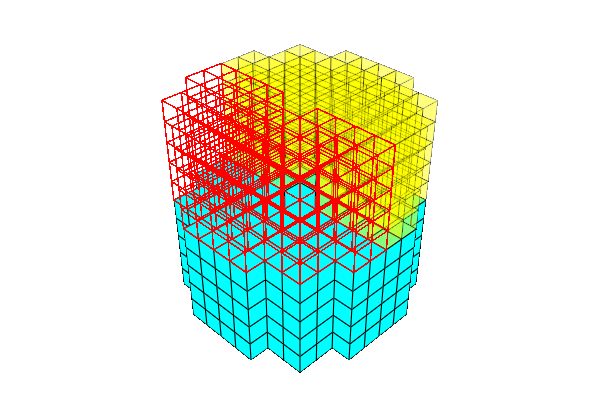
We are about to build a compound mesh by transforming parts of a voxlized cylinder into tetrahedra and lines. Then we do some plotting and review the basics of configuring plots.

from sigmaepsilon.mesh.space import CartesianFrame
from sigmaepsilon.mesh.recipes import cylinder
from sigmaepsilon.mesh import PolyData, LineData, PointData
from sigmaepsilon.mesh.cells import H8, Q4, L2
from sigmaepsilon.mesh.utils.topology import H8_to_L2, H8_to_Q4
from sigmaepsilon.mesh.utils.topology import detach_mesh_bulk
from sigmaepsilon.mesh.utils.space import frames_of_lines, frames_of_surfaces
from sigmaepsilon.math import minmax
import numpy as np

min_radius = 5
max_radius = 25
h = 50
angle = 1

shape = (min_radius, max_radius), angle, h
frame = CartesianFrame(dim=3)
cyl = cylinder(shape, size=5.0, voxelize=True, frame=frame)

coords = cyl.coords()
topo = cyl.topology().to_numpy()
centers = cyl.centers()

cxmin, cxmax = minmax(centers[:, 0])
czmin, czmax = minmax(centers[:, 2])
cxavg = (cxmin + cxmax) / 2
czavg = (czmin + czmax) / 2
b_upper = centers[:, 2] > czavg
b_lower = centers[:, 2] <= czavg
b_left = centers[:, 0] < cxavg
b_right = centers[:, 0] >= cxavg
iL2 = np.where(b_upper & b_right)[0]
iTET4 = np.where(b_upper & b_left)[0]
iH8 = np.where(b_lower)[0]
_, tL2 = H8_to_L2(coords, topo[iL2])
_, tQ4 = H8_to_Q4(coords, topo[iTET4])
tH8 = topo[iH8]

pd = PointData(coords=coords, frame=frame)
mesh = PolyData(pd, frame=frame)

cdL2 = L2(topo=tL2, frames=frames_of_lines(coords, tL2))
mesh["lines", "L2"] = LineData(cdL2, frame=frame)

cdQ4 = Q4(topo=tQ4, frames=frames_of_surfaces(coords, tQ4))
mesh["surfaces", "Q4"] = PolyData(cdQ4, frame=frame)

cH8, tH8 = detach_mesh_bulk(coords, tH8)
pdH8 = PointData(coords=cH8, frame=frame)
cdH8 = H8(topo=tH8, frames=frame)
mesh["bodies", "H8"] = PolyData(pdH8, cdH8, frame=frame)

mesh.to_standard_form()
mesh.lock(create_mappers=True)

PolyData({'frame': Array([[1., 0., 0.],
       [0., 1., 0.],
       [0., 0., 1.]]), 'lines': PolyData({'L2': PolyData({'frame': Array([[1., 0., 0.],
       [0., 1., 0.],
       [0., 0., 1.]])})}), 'surfaces': PolyData({'Q4': PolyData({'frame': Array([[1., 0., 0.],
       [0., 1., 0.],
       [0., 0., 1.]])})}), 'bodies': PolyData({'H8': PolyData({'frame': Array([[1., 0., 0.],
       [0., 1., 0.],
       [0., 0., 1.]])})})})

Add some configuration to the PyVista plotting mechanism. This requires to think about a config_key, that later we can use to point at our configuration. The configurations are stored in the config attribute of each block we are about to plot. For example, to set some basic properties:

mesh["lines", "L2"].config["pyvista", "plot", "color"] = "red"
mesh["lines", "L2"].config["pyvista", "plot", "line_width"] = 1.5
mesh["lines", "L2"].config["pyvista", "plot", "render_lines_as_tubes"] = True

mesh["surfaces", "Q4"].config["pyvista", "plot", "show_edges"] = True
mesh["surfaces", "Q4"].config["pyvista", "plot", "color"] = "yellow"
mesh["surfaces", "Q4"].config["pyvista", "plot", "opacity"] = 0.3

mesh["bodies", "H8"].config["pyvista", "plot", "show_edges"] = True
mesh["bodies", "H8"].config["pyvista", "plot", "color"] = "cyan"
mesh["bodies", "H8"].config["pyvista", "plot", "opacity"] = 1.0

The following block shows how to refer to the previously set config.

mesh.pvplot(
    notebook=True,
    jupyter_backend="static",
    cmap="plasma",
    window_size=(600, 400),
    config_key=["pyvista", "plot"],
    theme="document",
)