Plotting#
The library has a group of conviniance functions for plotting with various backends. The goal here is to collect functions for the most popular plotting libraries that work well out of the box for the majority of cases and provide options for fine tuning. If you want more control over your plots, you should use these libraries directly.
Plotting with Matplotlib#
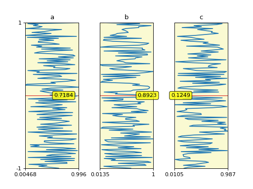
- sigmaepsilon.mesh.plotting.mpl.aligned_parallel_mpl(data: ndarray | dict, datapos: Iterable[float], *, yticks=None, labels=None, sharelimits=False, texlabels=None, xticksrotation=0, suptitle=None, slider=False, slider_label=None, hlines=None, vlines=None, y0=None, xoffset=0.0, yoffset=0.0, return_figure: bool | None = True, wspace: float | None = 0.4, **kwargs) Figure | None[source]#
- Parameters:
data (numpy.ndarray or dict) – The values to plot. If it is a NumPy array, labels must be provided with the argument labels, if it is a sictionary, the keys of the dictionary are used as labels.
datapos (Iterable[float]) – Positions of the provided data values.
yticks (Iterable[float], Optional) – Positions of ticks on the vertical axes. Default is None.
labels (Iterable, Optional) – An iterable of strings specifying labels for the datasets. Default is None.
sharelimits (bool, Optional) – If True, the axes share limits of the vertical axes. Default is False.
texlabels (Itrable[str], Optional) – TeX-formatted labels. If provided, it must have the same length as labels. Default is None.
xticksrotation (int, Optional) – Rotation of the ticks along the vertical axes. Expected in degrees. Default is 0.
suptitle (str, Optional) – See Matplotlib’s docs for the details. Default is None.
slider (bool, Optional) – If True, a slider is added to the figure for interactive plots. Default is False.
slider_label (str, Optional) – A label for the slider. Only if slider is true. Default is None.
hlines (Iterable[float], Optional) – A list of data values where horizontal lines are to be added to the axes. Default is None.
vlines[float] (Iterable, Optional) – A list of data values where vertical lines are to be added to the axes. Default is None.
y0 (float or int, Optional) – Value for the vertical axis. Default is the average of the limits of the vertical axis (0.5*(datapos[0] + datapos[-1])).
xoffset (float, Optional) – Margin of the plot in the vertical direction. Default is 0.
yoffset (float, Optional) – Margin of the plot in the horizontal direction. Default is 0.
wspace (float, Optional) – Spacing between the axes. Default is 0.4.
**kwargs (dict, Optional) – Extra keyword arguments are forwarded to the creator of the matplotlib figure. Default is None.
Example
from sigmaepsilon.mesh.plotting.mpl.parallel import aligned_parallel_mpl
import numpy as np
labels = ['a', 'b', 'c']
values = np.array([np.random.rand(150) for _ in labels]).T
datapos = np.linspace(-1, 1, 150)
aligned_parallel_mpl(values, datapos, labels=labels, yticks=[-1, 1], y0=0.0)
(
Source code,png,hires.png,pdf)
- sigmaepsilon.mesh.plotting.mpl.decorate_mpl_ax(*, fig=None, ax=None, aspect='equal', xlim=None, ylim=None, axis='on', offset=0.05, points=None, axfnc: Callable | None = None, title=None, suptitle=None, label=None)[source]#
Decorates an axis using the most often used modifiers.
- sigmaepsilon.mesh.plotting.mpl.parallel_mpl(data: dict | Iterable[ndarray] | ndarray, *, labels: Iterable[str] | None = None, padding: float | None = 0.05, colors: Iterable[str] | None = None, lw: float | None = 0.2, bezier: bool | None = True, figsize: tuple | None = None, title: str | None = None, ranges: Iterable[float] | None = None, return_figure: bool | None = True, **_) Figure | None[source]#
- Parameters:
data (Union[Iterable[numpy.ndarray], dict, numpy.ndarray]) – A list of numpy.ndarray for each column. Each array is 1d with a length of N, where N is the number of data records (the number of lines).
labels (Iterable, Optional) – Labels for the columns. If provided, it must have the same length as data.
padding (float, Optional) – Controls the padding around the axes.
colors (list of float, Optional) – A value for each record. Default is None.
lw (float, Optional) – Linewidth.
bezier (bool, Optional) – If True, bezier curves are created instead of a linear polinomials. Default is True.
figsize (tuple, Optional) – A tuple to control the size of the figure. Default is None.
title (str, Optional) – The title of the figure.
ranges (list of list, Optional) – Ranges of the axes. If not provided, it is inferred from the input values, but this may result in an error. Default is False.
return_figure (bool, Optional) – If True, the figure is returned. Default is False.
Example
from sigmaepsilon.mesh.plotting import parallel_mpl
import numpy as np
colors = np.random.rand(150, 3)
labels = [str(i) for i in range(10)]
values = [np.random.rand(150) for i in range(10)]
parallel_mpl(
    values,
    labels=labels,
    padding=0.05,
    lw=0.2,
    colors=colors,
    title="Parallel Plot with Random Data",
)
(
Source code,png,hires.png,pdf)
- sigmaepsilon.mesh.plotting.mpl.triplot_mpl_data(triobj: Any, data: ndarray | None, *_, fig: Figure | None = None, ax: Axes | Iterable[Axes] | None = None, cmap: str | None = 'jet', ecolor: str | None = 'k', lw: float | None = 0.1, title: str | None = None, suptitle: str | None = None, label: str | None = None, nlevels: int | None = None, refine: bool | None = False, refiner: Any | None = None, colorbar: bool | None = True, subdiv: int | None = 3, cbpad: str | None = '2%', cbsize: str | None = '5%', cbpos: str | None = 'right', draw_contours: bool | None = True, shading: str | None = 'flat', contour_colors: str | None = 'auto', **kwargs) Any[source]#
Convenience function to plot data over triangulations using matplotlib. Depending on the arguments, the function calls matplotlib.pyplot.tricontourf (optionally followed by matplotlib.pyplot.tricontour) or matplotlib.pyplot.tripcolor.
- Parameters:
triobj ('TriangulationLike') – This is either a tuple of mesh data (coordinates and topology) or a triangulation object understood by :func:~`sigmaepsilon.mesh.triang.triangulate`.
data (numpy.ndarray, Optional) – Some data to plot as an 1d or 2d NumPy array.
fig (matplotlib.figure.Figure, Optional) – A matplotlib figure to plot on. Default is None.
ax (matplotlib.axes.Axes or Iterable[matplotlib.axes.Axes], Optional.) – A matplotlib axis or more if data is 2 dimensional. Default is None.
cmap (str, Optional) – The name of a colormap. The default is ‘jet’.
ecolor (str, Optional) – The color of the edges of the triangles. This is only used if data is provided over the cells. Default is ‘k’.
lw (Number, Optional) – The linewidth. This is only used if data is provided over the cells. Default is 0.1.
title (str, Optional) – Title of the plot. See matplotlib for further details. Default is None.
suptitle (str, Optional) – The subtitle of the plot. See matplotlib for further details. Default is None.
label (str or Iterable[str], Optional) – The label of the axis or more labels if data is 2 dimensional and there are more axes. See matplotlib for further details. Default is None.
nlevels (int, Optional) – Number of levels on the colorbar, only if colorbar is True. Default is None, in which case the colorbar has a continuous distribution. See the examples for the details.
refine (bool, Optional) – Wether to refine the values. Default is False.
refiner (Any, Optional) – A valid matplotlib refiner, only if refine is True. If not specified, a UniformTriRefiner is used. Default is None.
subdiv (int, Optional) – Number of subdivisions for the refiner, only if refine is True. Default is 3.
cbpad (str, Optional) – The padding of the colorbar. Default is “2%”.
cbpos (str, Optional) – The position of the colorbar. Default is “right”.
colorbar (bool, Optional) – Wether to put a colorbar or not. Default is False.
draw_contours (bool, Optional) – Wether to draw contour levels or not. Only if data is provided over the cells and nlevels is also specified. Default is True.
contour_colors (str, Optional) – The color of the contourlines, only if draw_contours is True. Default is ‘auto’, which means the same as is used for the plot.
shading (str, Optional) – Shading for matplotlib.pyplot.tripcolor, for the case if nlevels is None. Default is ‘flat’.
**kwargs** (dict, Optional) – The extra keyword arguments are forwarded to
decorate_mpl_ax().
See also
decorate_mpl_ax()Examples
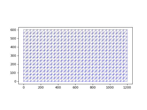
import numpy as np
from sigmaepsilon.mesh import grid
from sigmaepsilon.mesh.utils.topology.tr import Q4_to_T3
from sigmaepsilon.mesh import triangulate
from sigmaepsilon.mesh.plotting.mpl.triplot import triplot_mpl_data

gridparams = {
    "size": (1200, 600),
    "shape": (30, 15),
    "eshape": (2, 2),
}
coordsQ4, topoQ4 = grid(**gridparams)
points, triangles = Q4_to_T3(coordsQ4, topoQ4, path="grid")
triobj = triangulate(points=points[:, :2], triangles=triangles)[-1]

# Data defined over the triangles
data = np.random.rand(len(triangles))
triplot_mpl_data(triobj, data=data)

# Data defined over the points
data = np.random.rand(len(points))
triplot_mpl_data(
    triobj, data=data, cmap="jet", nlevels=10, refine=True, draw_contours=True
)


- sigmaepsilon.mesh.plotting.mpl.triplot_mpl_hinton(triobj: Any, data: ndarray | None, *_, fig: Figure | None = None, ax: Axes | Iterable[Axes] | None = None, lw: float | None = 0.5, fcolor: str | None = 'b', ecolor: str | None = 'k', title: str | None = None, suptitle: str | None = None, label: str | None = None, **kwargs) Any[source]#
Creates a hinton plot of triangles. The idea is from this example from Matplotlib:
https://matplotlib.org/stable/gallery/specialty_plots/hinton_demo.html
- Parameters:
triobj ('TriangulationLike') – This is either a tuple of mesh data (coordinates and topology) or a triangulation object understood by :func:~`sigmaepsilon.mesh.triang.triangulate`.
data (numpy.ndarray, Optional) – Some data to plot as an 1d NumPy array.
fig (matplotlib.figure.Figure, Optional) – A matplotlib figure to plot on. Default is None.
ax (matplotlib.axes.Axes or Iterable[matplotlib.axes.Axes], Optional.) – A matplotlib axis or more if data is 2 dimensional. Default is None.
ecolor (str, Optional) – The color of the edges of the original triangles, before scaling. Default is ‘k’.
fcolor (str, Optional) – The color of the triangles. Default is ‘b’.
lw (Number, Optional) – The linewidth. Default is 0.5.
title (str, Optional) – Title of the plot. See matplotlib for further details. Default is None.
suptitle (str, Optional) – The subtitle of the plot. See matplotlib for further details. Default is None.
label (str or Iterable[str], Optional) – The label of the axis. Default is None.
**kwargs** (dict, Optional) – The extra keyword arguments are forwarded to
decorate_mpl_ax().
See also
decorate_mpl_ax()Example
import numpy as np
from sigmaepsilon.mesh import grid
from sigmaepsilon.mesh.utils.topology.tr import Q4_to_T3
from sigmaepsilon.mesh import triangulate
from sigmaepsilon.mesh.plotting.mpl.triplot import triplot_mpl_hinton

gridparams = {
    "size": (1200, 600),
    "shape": (30, 15),
    "eshape": (2, 2),
}
coordsQ4, topoQ4 = grid(**gridparams)
points, triangles = Q4_to_T3(coordsQ4, topoQ4, path="grid")
triobj = triangulate(points=points[:, :2], triangles=triangles)[-1]

data = np.random.rand(len(triangles))
triplot_mpl_hinton(triobj, data=data)
(
Source code,png,hires.png,pdf)
- sigmaepsilon.mesh.plotting.mpl.triplot_mpl_mesh(triobj: Any, *_, fig: Figure | None = None, ax: Axes | None = None, lw: float | None = 0.5, marker: str | None = 'b-', zorder: int | None = None, fcolor: str | None = None, ecolor: str | None = 'k', title: str | None = None, suptitle: str | None = None, label: str | None = None, **kwargs) Any[source]#
Plots the mesh of a triangulation.
- Parameters:
triobj ('TriangulationLike') – This is either a tuple of mesh data (coordinates and topology) or a triangulation object understood by :func:~`sigmaepsilon.mesh.triang.triangulate`.
fig (matplotlib.figure.Figure, Optional) – A matplotlib figure to plot on. Default is None.
ax (matplotlib.axes.Axes or Iterable[matplotlib.axes.Axes], Optional.) – A matplotlib axis or more if data is 2 dimensional. Default is None.
ecolor (str, Optional) – The color of the edges of the original triangles, before scaling. Default is ‘k’.
fcolor (str, Optional) – The color of the triangles. Default is ‘b’.
lw (Number, Optional) – The linewidth. Default is 0.5.
zorder (int, Optional) – The zorder of the plot. See matplotlib for further details. Default is None.
title (str, Optional) – Title of the plot. See matplotlib for further details. Default is None.
suptitle (str, Optional) – The subtitle of the plot. See matplotlib for further details. Default is None.
label (str or Iterable[str], Optional) – The label of the axis. Default is None.
**kwargs** (dict, Optional) – The extra keyword arguments are forwarded to
decorate_mpl_ax().
See also
decorate_mpl_ax()Example
from sigmaepsilon.mesh import grid
from sigmaepsilon.mesh.utils.topology.tr import Q4_to_T3
from sigmaepsilon.mesh import triangulate
from sigmaepsilon.mesh.plotting.mpl.triplot import triplot_mpl_mesh

gridparams = {
    "size": (1200, 600),
    "shape": (30, 15),
    "eshape": (2, 2),
}
coordsQ4, topoQ4 = grid(**gridparams)
points, triangles = Q4_to_T3(coordsQ4, topoQ4, path="grid")
triobj = triangulate(points=points[:, :2], triangles=triangles)[-1]

triplot_mpl_mesh(triobj)
(
Source code,png,hires.png,pdf)
Plotting with Plotly#
- sigmaepsilon.mesh.plotting.plotly.plot_lines_plotly(coords: ndarray, topo: ndarray, *args, scalars: ndarray | None = None, fig: Figure | None = None, marker_symbol: str = 'circle', **kwargs) Figure[source]#
Plots points and lines in 3d space optionally with data defined on the points. If data is provided, the values are shown in a tooltip when howering above a point.
- Parameters:
coords (numpy.ndarray) – The coordinates of the points, where the first axis runs along the points, the second along spatial dimensions.
topo (numpy.ndarray) – The topology of the lines, where the first axis runs along the lines, the second along the nodes.
scalars (numpy.ndarray) – The values to show in the tooltips of the points as a 1d or 2d NumPy array. The length of the array must equal the number of points. Default is None.
marker_symbol (str, Optional) – The symbol to use for the points. Refer to Plotly’s documentation for the possible options. Default is “circle”.
Example
from sigmaepsilon.mesh.plotting import plot_lines_plotly
from sigmaepsilon.mesh import grid
from sigmaepsilon.mesh.utils.topology.tr import H8_to_L2
import numpy as np
gridparams = {
    "size": (10, 10, 10),
    "shape": (4, 4, 4),
    "eshape": "H8",
}
coords, topo = grid(**gridparams)
coords, topo = H8_to_L2(coords, topo)
data = np.random.rand(len(coords), 2)
plot_lines_plotly(coords, topo, scalars=data, scalar_labels=["X", "Y"])
(Source code, html)
- sigmaepsilon.mesh.plotting.plotly.scatter_points_plotly(coords: ndarray | None, *, scalars: ndarray | None = None, markersize: Number | None = 1, scalar_labels: Iterable[str] | None = None) Figure[source]#
Convenience function to plot several points in 3d with data and labels.
- Parameters:
coords (numpy.ndarray) – The coordinates of the points, where the first axis runs along the points, the second along spatial dimensions.
scalars (numpy.ndarray) – The values to show in the tooltips of the points as a 1d or 2d NumPy array. The length of the array must equal the number of points. Default is None.
markersize (int, Optional) – The size of the balls at the point coordinates. Default is 1.
scalar_labels (Iterable[str], Optional) – The labels for the columns in ‘scalars’. Default is None.
Example
from sigmaepsilon.mesh.plotting import scatter_points_plotly
import numpy as np
points = np.array([
    [0, 0, 0],
    [1, 0, 0],
    [0, 1, 0],
    [0, 0, 1]
])
data = np.random.rand(len(points))
scalar_labels=["random data"]
scatter_points_plotly(points, scalars=data, scalar_labels=scalar_labels)
(Source code, html)
- sigmaepsilon.mesh.plotting.plotly.triplot_plotly(points: ndarray, triangles: ndarray, data: ndarray | None = None, plot_edges: bool | None = True, edges: bool | None = None) Figure[source]#
Plots a triangulation optionally with edges and attached field data in 3d.
- Parameters:
points (numpy.ndarray) – 2d float array of points.
data (numpy.ndarray) – 1d float array of scalar data over the points.
plot_edges (bool, Optional) – If True, plots the edges of the mesh. Default is False.
edges (numpy.ndarray, Optional) – The edges to plot. If provided, plot_edges is ignored. Default is None.
- Returns:
figure – The figure object.
- Return type:
plotly.graph_objects.Figure
Example
from sigmaepsilon.mesh.plotting import triplot_plotly
from sigmaepsilon.mesh import grid
from sigmaepsilon.mesh.utils.topology.tr import Q4_to_T3
import numpy as np
gridparams = {
    "size": (1200, 600),
    "shape": (4, 4),
    "eshape": (2, 2),
}
coords, topo = grid(**gridparams)
points, triangles = Q4_to_T3(coords, topo, path="grid")
data = np.random.rand(len(points))
triplot_plotly(points, triangles, data, plot_edges=True)
(Source code, html)
Plotting with PyVista#
- sigmaepsilon.mesh.plotting.pvplot.pvplot(obj: PolyData, *, deepcopy: bool = False, jupyter_backend: str = 'pythreejs', show_edges: bool = True, notebook: bool = False, theme: str | None = None, scalars: str | ndarray | None = None, window_size: Tuple | None = None, return_plotter: bool = False, config_key: Tuple | None = None, plotter: Plotter | None = None, cmap: str | Iterable | None = None, camera_position: Tuple | None = None, lighting: bool = False, edge_color: str | None = None, return_img: bool = False, show_scalar_bar: bool | None = None, opacity: float | None = None, style: str | None = None, add_legend: bool = False, legend_params: dict | None = None, **kwargs) None | Plotter | ndarray[source]#
Plots the mesh using PyVista. The parameters listed here only grasp a fraction of what PyVista provides. The idea is to have a function that narrows down the parameters as much as possible to the ones that are most commonly used. If you want more control, create a plotter prior to calling this function and provide it using the parameter plotter. Then by setting return_plotter to True, the function adds the cells to the plotter and returns it for further customization.
- Parameters:
deepcopy (bool, Optional) – If True, a deep copy is created. Default is False.
jupyter_backend (str, Optional) – The backend to use when plotting in a Jupyter enviroment. Default is ‘pythreejs’.
show_edges (bool, Optional) – If True, the edges of the mesh are shown as a wireframe. Default is True.
notebook (bool, Optional) – If True and in a Jupyter enviroment, the plot is embedded into the Notebook. Default is False.
theme (str, Optional) – The theme to use with PyVista. Default is None.
scalars (Union[str, numpy.ndarray]) – A string that refers to a field in the celldata objects of the block of the mesh, or a NumPy array with values for each point in the mesh.
window_size (tuple, Optional) – The size of the window, only is notebook is False. Default is None.
return_plotter (bool, Optional) – If True, an instance of
pyvista.Plotteris returned without being shown. Default is False.config_key (tuple, Optional) – A tuple of strings that refer to a configuration for PyVista.
plotter (pyvista.Plotter, Optional) – A plotter to use. If not provided, a plotter is created in the background. Default is None.
cmap (Union[str, Iterable], Optional) – A color map for plotting. See PyVista’s docs for the details. Default is None.
camera_position (tuple, Optional) – Camera position. See PyVista’s docs for the details. Default is None.
lighting (bool, Optional) – Whether to use lighting or not. Default is None.
edge_color (str, Optional) – The color of the edges if show_edges is True. Default is None, which equals to the default PyVista setting.
return_img (bool, Optional) – If True, a screenshot is returned as an image. Default is False.
show_scalar_bar (Union[bool, None], Optional) – Whether to show the scalar bar or not. A None value means that the option is governed by the configurations of the blocks. If a boolean is provided here, it overrides the configurations of the blocks. Default is None.
opacity (float, Optional) – The opacity of the mesh. Default is None. .. versionadded:: 3.1.0
style (str, Optional) – Visualization style of the mesh. Default is None. .. versionadded:: 3.1.0
add_legend (bool, Optional) – If True, a legend is added to the plot. Default is False. .. versionadded:: 3.1.0
legend_params (dict, Optional) – Parameters for the legend to be forwarded to the function
pyvista.Plotter.add_legend(). Default is None. .. versionadded:: 3.1.0**kwargs – Extra keyword arguments passed to pyvista.Plotter, if the plotter has to be created.
- Returns:
A PyVista plotter if return_plotter is True, a NumPy array if return_img is True, or nothing.
- Return type:
Union[None, pv.Plotter, numpy.ndarray]
Example
from sigmaepsilon.mesh.plotting import pvplot
from sigmaepsilon.mesh.downloads import download_gt40
import matplotlib.pyplot as plt
mesh = download_gt40(read=True)
img=pvplot(mesh, notebook=False, return_img=True)
plt.imshow(img)
plt.axis('off')
(
Source code,png,hires.png,pdf)
Plotting with K3D#
- sigmaepsilon.mesh.plotting.k3dplot.k3dplot(obj: PolyData, scene: Plot | None = None, *, menu_visibility: bool | None = True, **kwargs) Plot[source]#
Plots the mesh using ‘k3d’ as the backend.
Warning
During this call there is a UserWarning saying ‘Given trait value dtype “float32” does not match required type “float32”’. Although this is weird, plotting seems to be just fine.
- Parameters:
scene (object, Optional) – A K3D plot widget to append to. This can also be given as the first positional argument. Default is None, in which case it is created using a call to
k3d.plot().menu_visibility (bool, Optional) – Whether to show the menu or not. Default is True.
**kwargs (dict, Optional) – Extra keyword arguments forwarded to
to_k3d().
Example
Get a compound mesh, add some random data to it and plot it with K3D.
# doctest: +SKIP

from sigmaepsilon.mesh.plotting import k3dplot
from sigmaepsilon.mesh.examples import compound_mesh
from k3d.colormaps import matplotlib_color_maps
import k3d
import numpy as np
mesh = compound_mesh()
cd_L2 = mesh["lines", "L2"].cd
cd_Q4 = mesh["surfaces", "Q4"].cd
cd_H8 = mesh["bodies", "H8"].cd
cd_L2.db["scalars"] = 100 * np.random.rand(len(cd_L2))
cd_Q4.db["scalars"] = 100 * np.random.rand(len(cd_Q4))
cd_H8.db["scalars"] = 100 * np.random.rand(len(cd_H8))
scalars = mesh.pd.pull("scalars")
cmap = matplotlib_color_maps.Jet
fig = k3d.plot()
k3dplot(mesh, fig, scalars=scalars, menu_visibility=False, cmap=cmap)
fig